
**I. Overview of the Least Mean Square Algorithm (LMS)**
In 1959, Widrow and Hoff introduced the Least Mean Square (LMS) algorithm while researching adaptive linear elements for pattern recognition. The LMS algorithm is based on Wiener filtering but uses the steepest descent method to approximate the Wiener solution iteratively. Unlike the Wiener filter, which requires prior statistical knowledge of the input and desired signals, the LMS algorithm avoids matrix inversion by using instantaneous error instead of mean square error. This makes it more practical for real-time applications.
The LMS algorithm is known for its low computational complexity, good convergence in stationary environments, and unbiased convergence toward the Wiener solution. It is stable even with limited precision, making it one of the most widely used adaptive algorithms.
The following figure illustrates the vector signal flow of the LMS algorithm:
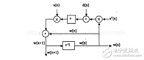
Figure 1: LMS Algorithm Vector Signal Flow
As shown in Figure 1, the LMS algorithm involves two main processes: filtering and weight adaptation. The general steps are as follows: 1. **Determine Parameters**: Choose a global step size parameter β and the number of filter taps (filter order). 2. **Initialize Weights**: Set initial values for the filter coefficients. 3. **Algorithm Operation**: - Filtered output: $ y(n) = w^T(n)x(n) $ - Error signal: $ e(n) = d(n) - y(n) $ - Weight update: $ w(n+1) = w(n) + \beta e(n)x(n) $ **II. Performance Analysis** The performance of an adaptive algorithm largely determines the effectiveness of the adaptive filter. Key performance metrics include convergence, convergence speed, steady-state error, and computational complexity. 1. **Convergence** Convergence refers to how well the filter weights approach the optimal value as the number of iterations increases. A convergent algorithm ensures that the weights eventually reach or remain close to the optimal solution. 2. **Convergence Speed** This measures how quickly the algorithm reaches the optimal solution from its initial state. Faster convergence is generally preferred in real-time applications. 3. **Steady-State Error** Once the algorithm has converged, the steady-state error represents the deviation between the current weights and the optimal weights. Lower steady-state error indicates better performance. 4. **Computational Complexity** This refers to the amount of computation required per iteration. The LMS algorithm is computationally efficient, making it ideal for resource-constrained systems. **III. Classification of the LMS Algorithm** 1. **Quantization Error LMS Algorithm** To reduce computational load, especially in high-speed applications like echo cancellation, the quantization error LMS algorithm quantizes the error signal. This reduces the number of operations needed during weight updates. 2. **De-correlated LMS Algorithm** The standard LMS assumes that input samples are statistically independent. When this assumption fails, convergence slows down. De-correlation techniques, such as time-domain or transform-domain methods, help improve convergence speed. 3. **Parallel Delay LMS Algorithm** This version is designed for VLSI implementations, offering high parallelism. However, delays introduced during processing can degrade convergence performance, especially for long filters. 4. **Adaptive Lattice LMS Algorithm** Unlike traditional LMS, which assumes a fixed filter order, the lattice LMS allows for dynamic order adjustment. This makes it more flexible in scenarios where the optimal filter order is unknown. 5. **Newton-LMS Algorithm** This variant uses second-order statistics to accelerate convergence, particularly when input signals are highly correlated. However, it requires inverting the input correlation matrix, which can be computationally intensive and numerically unstable. Overall, the LMS algorithm remains a cornerstone in adaptive signal processing due to its simplicity, efficiency, and robustness in various applications.Lead free Solder Bar is a solid solder bar,without flux, It was strictly following RoHS .WEEE directive and ISO14000 management system requirement
Product Brand:SnCu0.7.SnCu0.3.SnCu3.SnAg0.5Cu0.5.SnAg3Cu.SnAg4Cu.Sn Cu1Ag.
Sn Cu4Ag1.Sn Cu6Ag2.Sn Sb5
Lead Free Solder Bar,Silver Solder Bar,Solder Bar,Hot Bar Soldering
Shaoxing Tianlong Tin Materials Co.,Ltd. , https://www.tianlongspray.com