When the oscilloscope user performs the vertical quantity measurement such as amplitude/peak, the measurement result is slightly deviated from the expected result, and the measurement is not accurate enough, which makes the user question the measurement accuracy of the oscilloscope. Here, the oscilloscope amplitude/ Why is the measurement deviation occurring in the vertical measurement such as the peak value, and how this phenomenon will be improved to reduce the measurement error.
When the customer uses an oscilloscope to measure the vertical value such as the amplitude/peak value of high-frequency signals, strong voltages, small signals, or power supply ripples, noise, etc., the measured values ​​are deviated, and the measured values ​​of the vertical quantities are too small or too large, resulting in user-to-user Oscilloscope measurement accuracy is questionable.
Figure 1 Oscilloscope measurement question
The reason for the deviation of the oscilloscope vertical quantity measurement is summarized as the following four points:
1 Low frequency compensation adjustment or not;
2 The influence of the oscilloscope's noise floor interference on the measurement;
3 Differences in the amplitude-frequency characteristic curve of the oscilloscope;
4 The effect of the oscilloscope's vertical resolution on the measurement.
Of course, the oscilloscope measurement accuracy is not necessarily comparable to a high-precision multimeter. Therefore, if you want to measure more accurate data in the oscilloscope vertical quantity measurement, you need to master the correct operation skills.
1, low frequency compensation adjustment or notLow frequency compensation (LFC) requires the use of a square wave in the kHz range (usually 1 kHz or 10 kHz) to adjust the frequency response of the X10 probe. When performing low frequency compensation, use the probe to connect the kHz square wave signal. If there is over compensation or under compensation, you can use the low frequency adjustment rod to adjust the low frequency compensation capacitance of the probe to the square wave flat top.
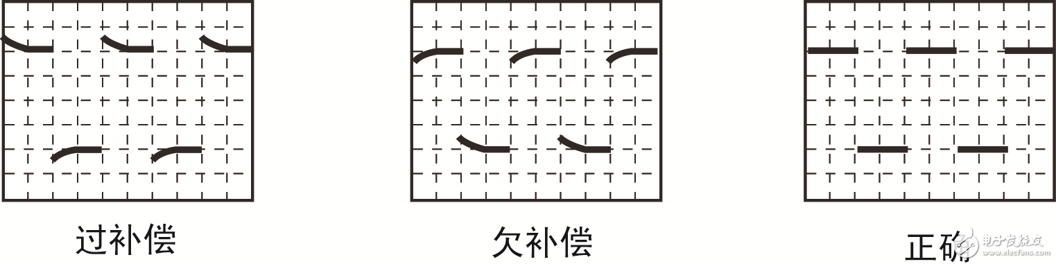
Figure 2 waveform compensation
Why do you have to compensate for low frequency?
Figure 3 below shows the internal circuit diagram when the probe is connected to the input of the oscilloscope. R1 is a 9MΩ serial Resistor, and a 10:1 attenuator is formed with the 1MΩ input resistor at the input of the oscilloscope, which can effectively reduce the input capacitance and is beneficial to high. Measurement of frequency signals.
When using the X10 probe to measure the signal, as the signal frequency increases, the influence of the capacitive load becomes more obvious. At this time, the parasitic capacitance (Cp, Cc) of the probe and cable in the probe body will cause the impedance of the probe and the oscilloscope to be mismatched. (R1xC1≠R2x(C2+Cc)), which affects signal measurement.
Due to the inconsistency of the parasitic capacitance, it is necessary to make C1 a tunable capacitor to compensate for the influence of parasitic capacitance, so that R1xC1=R2x(C2+Cc), so that the probe and the oscilloscope can be matched. Since the resistance values ​​of R1 and R2 are relatively large, the pole frequencies formed by R1, C1, R2, and C2 are relatively low, so this capacitance is also called a low frequency compensation capacitor.
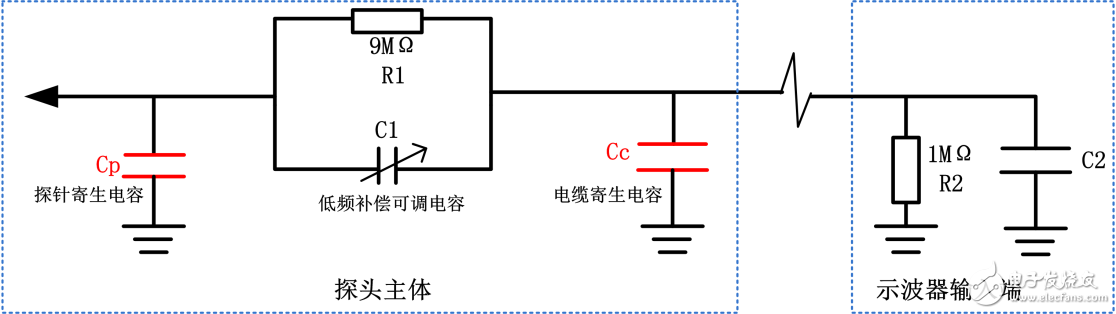
Figure 3 probe compensation circuit
The effect of low frequency compensation on the measurement of signal vertical quantity:
Taking the peak-to-peak value of the sine wave as an example, in the case of under-compensation, the vertical amount of the waveform will be too small. In the case of over-compensation, the vertical amount will be too large, as shown in Figure 4 below.
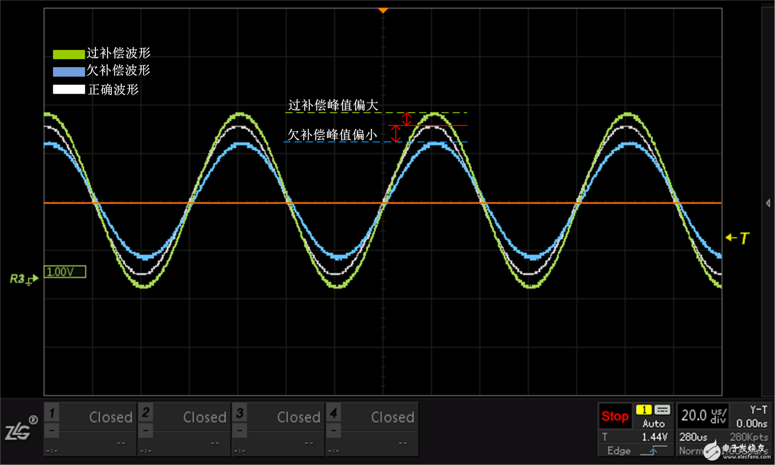
Figure 4 Variation of waveform amplitude under different compensation
2. The influence of the noise of the oscilloscope's noise floor on the measurementBottom noise:
Usually refers to the oscilloscope's “baseline noise floorâ€, the vertical noise caused by the analog front end of the oscilloscope and the digital conversion process. The magnitude of the noise floor is represented by the signal-to-noise ratio. The larger the value, the smaller the noise interference representing the signal, that is, the lower the noise floor of the measuring instrument.
The effect of noise floor on vertical measurement:
The noise floor appears on the oscilloscope screen as the noise waveform produced when the oscilloscope is placed in the most sensitive vertical gear . Of course, the oscilloscope's noise floor is related to the device, hardware design, signal processing and other aspects of the instrument, so the noise floor of different companies or different models of oscilloscopes is different, as shown in Figure 5.

Figure 5 Different companies have different oscilloscope noise levels
(1) When the oscilloscope's bottom noise is large, it will cover up the small signal, affecting the accuracy of the small signal measurement, resulting in inaccurate measurement vertical quantity;
(2) When the bottom noise of the oscilloscope is low, the measurement of the signal will be more accurate;
As shown in the example in Figure 6, the oscilloscope with a peak-to-peak value of 4mV is input to the oscilloscopes of two different companies, and the peak-to-peak value is measured separately to understand the influence of the noise floor on the measurement.
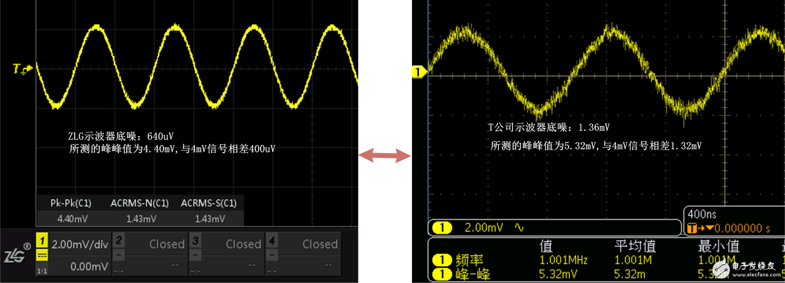
Figure 6 Comparison of oscilloscope peak-to-peak measurements of different companies
If you want to reduce the effect of noise floor noise on the measurement during measurement, you can use the following methods:
◠The oscilloscope's capture mode uses “average†capture. The average capture can average the multiple triggered periodic signals, making the signal slightly floating around a certain value, closer to the true value, to reduce the effects of noise.
◠The oscilloscope can use the “digital filtering†method to filter the noise signal larger than the cutoff frequency (less than the cutoff frequency) under low-pass filtering (high-pass filtering) to improve the accuracy of the measurement.
3. The amplitude-frequency characteristic curve of the oscilloscopeBandwidth: refers to the analog bandwidth of the oscilloscope's analog front end. Its size directly determines the range of signal bands that the oscilloscope can measure.
Specifically, the oscilloscope bandwidth refers to the highest frequency when the oscilloscope measures the amplitude of the sine wave not lower than the true sine wave signal -3dB amplitude (ie 70.7% of the true signal amplitude), also known as the -3dB cutoff frequency point. As the signal frequency increases, the oscilloscope's ability to accurately display the signal will decrease, as shown in Figure 7, which is the ideal amplitude-frequency characteristic curve.
The amplitude-frequency characteristic curve of the oscilloscope : refers to the curve of the amplitude of the oscilloscope signal as the signal frequency increases.
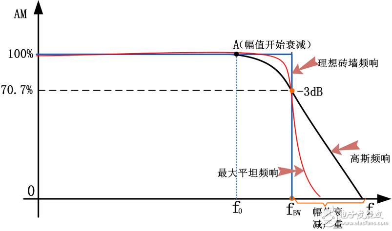
Figure 7 ideal amplitude frequency characteristic curve
As can be seen from Figure 7 above, when the frequency of the measured signal is equal to the bandwidth of the oscilloscope (fBW), the error of the amplitude measurement is about 30%. The amplitude of the signal frequency less than f0 is basically no attenuation. The signal starts to decay slowly between f0~fBW, and the attenuation of the signal is more serious than fBW. Therefore, if the attenuation of the signal amplitude is small, the frequency of the measured signal should be less than There are many values ​​for bandwidth.
Figure 8 shows the ideal amplitude-frequency characteristic curve, but the shape of the amplitude-frequency characteristic curve of the actual oscilloscope may not be ideal. The amplitude and frequency characteristics of different models of oscilloscopes may be different, but they will be as close as possible to the shape of the ideal curve.
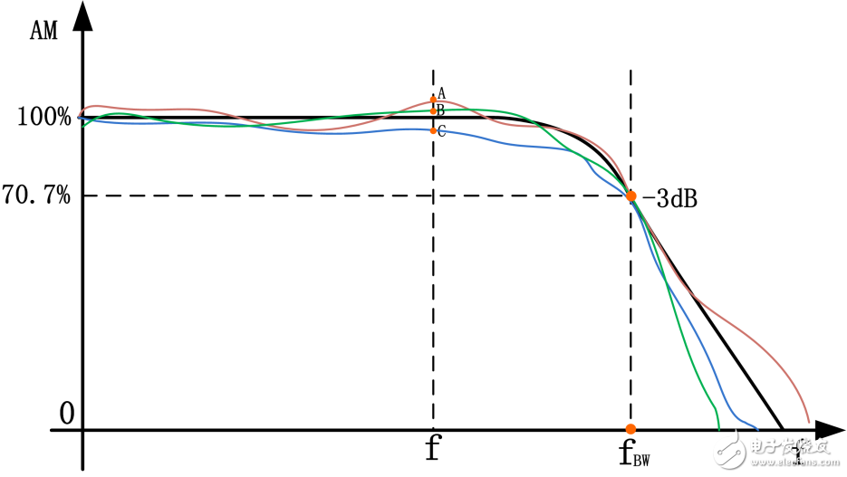
Figure 8 Actual amplitude-frequency characteristic curve
Figure 8 is a schematic diagram of the non-ideal amplitude-frequency characteristic curve. The different amplitude-frequency characteristics of different oscilloscopes have different flatness, but the in-band attenuation is within -3dB, which is in line with the standard. Therefore, the amplitude attenuation of signals of different oscilloscopes at the same frequency point may be different, which leads to the deviation of amplitude measurement by different oscilloscopes.
4, the impact of the vertical resolution of the oscilloscope on the measurementA typical digital oscilloscope uses an 8-bit ADC that recombines any of the waveform values ​​with 256 0's and 1's. Assume that the oscilloscope has a full-scale vertical range of 8 cells, corresponding to a quantization level of 256. In the case where the vertical scale is 500 mV/div, the vertical accuracy is (500 mV*8) / 256 = 15.625 mV. Measuring the same signal, with a vertical gear of 50mV/div, ie (50mV*8)/256=1.5625 mV, the vertical accuracy is 1.5625 mV.
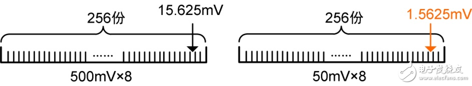
Figure 9 Measurement accuracy
In the actual measurement, since the amplitude of the measured waveform is different, the vertical gear setting will be different, but in order to make the measurement as accurate as possible, the following operations can be performed:
Make the test signal amplitude as much as possible to about 6 div of the screen. For example, a sine wave with a peak-to-peak value of 7Vpp should be set to 1V/div instead of 2V/div or 5V/div. In fact, this involves a voltage resolution problem, the ZDS4054 plus oscilloscope ADC has a quantized resolution of 25LSB/div. For example, at a voltage of 1V/div, the voltage resolution is 40mv, and when 10V/div, the voltage resolution is 400mv. It can be seen that at 1V/div, the measured value has a higher resolution and the measured value is more accurate.
In summary, the oscilloscope can observe the overall trend of waveform changes, the core is high bandwidth, high sampling rate, high refresh rate, and tends to high-speed signal measurement. High-precision multimeters and power analyzers are recommended for high-precision vertical measurement of low-speed signals.
Power Film Capacitors - Plastic Case
Polypropylene High Voltage Capacitor,axial film capacitor,axial capacitor,SHV capacitor
XIAN STATE IMPORT & EXPORT CORP. , https://www.capacitorhv.com